The Joy of Transformations of Functions

Last year, I was first called upon to teach a section our college algebra course, MATH 120. It was an interesting experience, to say the least, and it opened my eyes to a few beautiful elements of the subject that I had never noticed before.

My journey with algebra proper started and ended in junior high school. In fact, I believe that the last algebra course that I took was when I was in ninth grade. When I went to college, I started out right in calculus and never looked back. So, naturally, I didn’t have particularly high expectations for the content. “It’s just moving x around in equations, and that odd ‘completing the square’ thing that I haven’t done in years, surely,” I thought to myself. “Oh, and memorizing a bunch of random forms of specific equations that they’ll never use again… that too!”

And so it was with rather low expectations that I opened up an algebra text for the first time in a decade. It was Blitzer’s College Algebra Essentials, a book that the lead of the program had selected “because they all suck, and at least this one is cheap”. And, to be honest, the book itself lived up to every one of my low expectations.

But once I fought through the colorful pictures of unrelated television personalities and got to the mathematics itself, I discovered something very special.

Over the past few years, I’ve really started to appreciate my “computer science” brain. I don’t know where the point of inflection was, but at some point between when I started learning to program and today, my mind has adapted itself to working to rules and abstractions as almost a matter of course. And exposing this new mind of mine to a topic that I had, quite honestly, loathed back in junior high, produced unexpected results. I started noticing patterns.

Transformations of Functions: A Summary

Where everything started to come together for me was when I was reading over Blitzer’s section on Transformations of Functions. For those of you who have been out of algebra for as long as I had been, let me summarize these here.

The basic idea is that there are consistent arithmetic adjustments that you can make to functions that will allow you to alter the form of their graph. You can translate functions up and down, stretch them horizontally or vertically, and reflect them across the $x$ and $y$-axis. And, most importantly, these rules are extremely consistent. It doesn’t matter what the function is–these rules will work on it.

Horizontal Translation

Given a function, $f(x)$, I can translate the function horizontally by using $f(x - a)$. To give a specific example, consider the function, $$ f(x) = x^2 $$

I can create a new function, say $g(x)$, that is the same as $f$, except with every point shifted by $3$ units to the right along the $x$-axis, by doing the following, $$ g(x) = f(x - r) = (x - 3)^2 $$

Or, if I prefer, I can shift everything to the left by $3$ units instead to create $h(x)$. $$ h(x) = f(x - (-3)) = (x + 3)^2 $$

Figure 1, below, shows all three of these graphs, created using Geogebra.

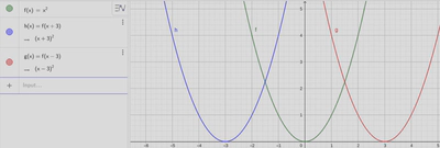
This rule makes a lot of sense. You can shift the graph horizontally, in other words along the $x$-axis, by adding or subtracting from the $x$ values. The only tricky part is that the directions are reversed from what one might expect: you subtract to move right and add to move left. But it does make sense once you tear into the actual numbers. I won’t spoil the joy of figuring out why it works, if you don’t already know. Take a moment and write out tables of $x$ and $y$ values for $f$, $g$, and $h$ above. If you study these closely, you might be able to determine what is going on!

Vertical Translation

For the case of vertical translation, I have actually adopted a different approach to teaching it compared to the standard. However, I’ll address this later and focus on the traditional approach used in Blitzer, and other algebra texts. We’ll discuss “my way” later.

Given a function $f(x)$, I can translate the function vertically by using $ f(x) + b$. To give a specific example, consider the function, $$ f(x) = x^2 $$

I can create a new function, say $i(x)$, that is the same as $f$, except with every point shifted by $3$ units up along the $y$-axis, by doing the following, $$ i(x) = f(x) + 3 = x^2 + 3 $$

I can also shift everything down by $3$ units instead to create $j(x)$, $$ j(x) = f(x) -3 = x^2 - 3 $$

Figure 2 shows the graphs of these three functions.

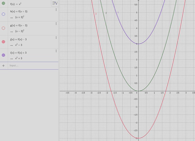
This rule also makes sense. It is a bit odd that the sign conventions are reversed compared to horizontal translations, but it does again seem reasonable that we can shift the graph vertically, along the $y$-axis, by adding/subtracting from the function itself (remember, we often say that $y=f(x)$.$y$ is just another name for $f$)

Horizontal Stretching

The stretching of the graph of a function is a lot harder to get a handle on. To be honest, it actually isn’t something that I require my students to learn outside of just exposure to the idea that it is accomplished by multiplication/division. However, I do want to discuss these here too–because they are useful to the discussion that I ultimately want to get to. So please bear with me as I fumble through attempting to explain these!

In order to really appreciate the difference between a horizontal and a vertical stretch, we need to examine the $x$ and $y$-intercepts of the function. So I’m going to transition to a different base function than the bare quadratic I’ve been using. For our horizontal stretching discussion, let’s consider $r(x) = (x)^2 - 1$. Yes, this function is a tad more complex, but it has $x$-intercepts for us to look at. These are critical for understanding the differences here.

When I “stretch” my function horizontally, I am going to take its $x$-intercepts and increase their magnitude (effectively spreading them apart, in the case of this parabola). I can accomplish this by dividing $x$ in my function by a constant. For example, if I wanted to double the magnitude of my $x$-intercepts, I would divide by $2$. So I can create a new function, $s(x)$, using,

$$ s(x) = r(x/2) = \left(\frac{x}{2}\right)^2 - 1 $$

If I multiply rather than dividing, then I can shrink the magnitude of (and, by extension, the distance between) my $x$-intercepts. So multiplying by $2$ is going to cut the magnitude of the intercepts of my function in half, creating $t(x)$, $$ t(x) = r(2x) = (2x)^2 - 1 $$

Hopefully, this figure will make these stretching/shrinking shenanigans a bit more clear. Figure 3 shows graphs of $r$, $s$, and $t$.

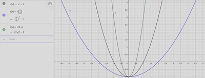
This figure warrants a bit of discussion. The $x$-intercepts of the “base” function, $r$, are located at $1$ and $-1$. When I divide x by 2, stretching horizontally, as in $s$, the coordinates of these intercepts double and we see intercepts of $2$ and $-2$ instead.

The same goes for the shrink, demonstrated by $t$. Multiplying by $2$ has the effect of cutting the intercepts in half. This function has intercepts at $0.5$ and $-0.5$.

Also, notice through all of this that our $y$-intercept has remained unchanged. A horizontal stretch will not change the $y$-intercept.

So, just to summarize here, you stretch or shrink the $x$-intercepts (a horizontal stretch/shrink) by multiplying/dividing $x$. To stretch and increase their magnitude, divide $x$, and to shrink and decrease their magnitude, multiply $x$.

Vertical Stretching

Next, we’ll do vertical stretching. This will move around our $y$-intercept, so let’s define a new function, $o(x) = (x+1)^2$, to use for our example. This will have a non-zero $y$-intercept so we can see what effects our stretching has.

First, we will do a vertical stretch. If we multiply $o(x)$ itself by two, this will double the value of the $y$-intercept. Thus, we construct $p(x)$, $$ p(x) = 2o(x) = 2(x+1)^2 $$

Notice that–just like with the horizontal vs. vertical translations, the rules are strangely reversed for horizontal and vertical stretches. A horizontal stretch requires dividing by the stretch factor, while a vertical one requires multiplying by the stretch factor. We’ll address this later.

Likewise, we can do a vertical shrink by dividing $o(x)$ itself by two. This will cut the value of the $y$-intercept in half. Let’s call this $q(x)$,

$$ q(x) = \frac{1}{2} o(x) = \frac{1}{2}(x+1)^2 $$

Graphing all three of these cases will give us Figure 4,

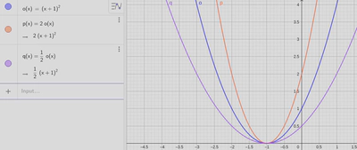
Notice that our base function has a $y$-intercept of $1$. Our stretching of this function by a factor of two properly doubles this intercept, moving it up to $2$, and shrinking by a factor of two cuts it in half, bringing it down to $0.5$. Note that, just like our horizontal stretch maintained the $y$-intercept, our vertical stretch maintained the $x$-intercepts.

Horizontal and Vertical Reflections

Finally, we can reflect the graph across the $x$ or $y$-axis. This is actually a special case of stretching, and occurs when we use a negative stretch factor. Let’s consider a sufficiently complex function to make this interesting, $$ a(x) = x^3 + 2x - 1 $$

We can reflect this graph horizontally by horizontally stretching it with a factor of $-1$. This will give us $b(x)$, $$ b(x) = a(-x) = (-x)^3 + 2(-x) -1 $$

And, likewise, we can flip it vertically by vertically stretching it with a factor of $-1$. Let’s call this one $c(x)$, $$ c(x) = -a(x) = -(x^3 + 2x - 1) $$

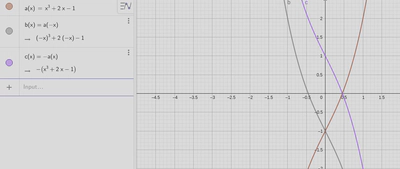
Figure 5 shows the results of these reflections. Let’s look at it in detail. Our “base” function, $a(x)$, has an $x$-intercept at just shy of $0.5$, and a $y$-intercept at $-1$. How did our reflections affect these intercepts?

Well, the horizontal reflection, shown by $b(x)$, reveals that the sign of our $x$-intercept flipped, while leaving the $y$-intercept the same. This basically follows the rules that we saw above with our stretches/shrinks. We multiplied the $x$-intercepts by our stretch factor, and left the $y$-intercepts alone.

The same story is reflected (no pun intended) in our vertical reflection in $c(x)$. Both $c(x)$ and $a(x)$ have the same $x$-intercept, however $c(x)$ has a $y$-intercept at $1$. The $y$-intercepts were flipped!

Note that this does lend itself to a somewhat backwards logic. A flipping of the $y$-intercepts is going to result in the graph reflecting across the $x$-axis, and a flipping of the $x$-intercepts will result in the graph reflecting across the $y$-axis. Again, there isn’t anything here that shouldn’t make sense once its been thought upon for a while–but it is odd and backwards at first glance.

Transformations of Equations

Okay–so I have just walked you through an (abbreviated) traditional approach to discussing this topic. I’m not fond of this approach because of the inconsistencies between the horizontal and vertical transformations. Why is it that these rules are reversed for the vertical ones, relative to the horizontal ones? And this approach also ties these transformations directly to functions, when they are far more powerful than that. We can apply these same transformations to many equations that are not functions at all!

So, I find that discussing these in the context of functions specifically is a bit limiting. What I do instead is consider them more generically–as applies to any equation of two variables, which I’ll call $x$ and $y$ in keeping with tradition. This has the double benefit of removing the artificial dependence on functional notation, and also removing the inconsistencies between vertical and horizontal transformations.

Here is what I do. First, I’ll recreate my translations, given $f(x) = x^2$.

The first step is to abandon the function notation and revert back to using $y$, $$ y = x^2 $$

When you do this, something magical happens. Remember how we could shift this graph up by $2$ by adding two to the end? $$ y = x^2 + 2 $$ $$ (y - 2) = x^2 $$

Hey! Look at that. Rather than using this odd backwards convention for vertical shifts, we can subtract from $y$. The same deal applies for the stretch/shrink situation. A vertical stretch was achieved by multiplying our function by $2$, $$ y = 2(x^2) $$ $$ \frac{1}{2} y = x^2 $$

We can revert this back to the exact same convention as a horizontal stretch if we look at it in terms of altering the $y$ variable, rather than the whole function.

What this gives us, in effect, is a very consistent set of rules,

1. For a horizontal translation, add to $x$ to move left and subtract from $x$ to move right.
2. For a vertical translation, add to $y$ to move down and subtract from $y$ to move up.
3. For a horizontal stretch, multiply $x$ to decrease the $x$-intercepts and divide $x$ to increase them.
4. For a vertical stretch, multiply $y$ to decrease the $y$-intercepts and divide $y$ to increase them.

The same rules now apply, where altering $x$ performs horizontal transformations, and altering $y$ performs vertical ones. In effect, we’ve cut the number of rules that need to be memorized in half!

Transformations of a Circle

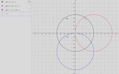
This scheme has the added benefit of allowing us to apply these rules easily to equations that are not functions. For example, consider the humble unit circle, $$ x^2 + y^2 = 1 $$

We can apply our translation rules to move this circle around where-ever we want! Figure 6 demonstrates this–the rules work for this! And they’ll work for other “non-functions” too, such as hyperbolas and square roots.

With circles specifically, something really cool happens when we start applying stretches. If we stretch it horizontally and vertically by the same amounts, then we increase the radius, as you might expect,

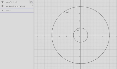
What is particularly neat here is that examining this result closely can show why it is that the radius in the standard form a circle is squared. If we do this in general terms, $$ \left( \frac{x}{R} \right)^2 + \left( \frac{y}{R} \right)^2 = 1 $$ $$ \frac{1}{R^2} \left( x^2 + y^2 \right) = 1 $$ $$ x^2 + y^2 = R^2 $$

Things get even neater when we start to apply asymmetrical stretches. What happens if we stretch horizontally and vertically by different amounts?

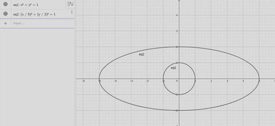
If we stretch horizontally by $a$ and vertically by $b$, then we end up with the general equation, $$ \left( \frac{x}{a} \right)^2 + \left( \frac{y}{b} \right)^2 = 1 $$ which you may recognize as the standard form of an ellipse. And we can derive it by simply starting with the “base” equation for the unit circle, and applying transformations.

Transformations of a Line

The standard form of most types of equation can be found by applying transformations like this. For example, consider a linear function, $$ f(x) = x $$ $$ y = x $$

We know that this graph will cross the point $(0,0)$. So, we can apply transformations to move this point anywhere we want. If we want to move that point that normally resides on the origin to a new location, $(x_1, y_1)$, then we can apply our translation rules to do this, $$ (y - y_1) = (x - x_1) $$

Next, let’s do our stretching. We will stretch horizontally by a factor called $\text{run}$ and vertically by a factor called $\text{rise}$. This will get us, $$ \frac{(y - y_1)}{\text{rise}} = \frac{(x - x_1)}{\text{run}} $$ $$ (y - y_1) = \frac{\text{rise}}{\text{run}} (x - x_1) $$ $$ (y - y_1) = m (x - x_1) $$ where $m = \frac{\text{rise}}{\text{run}}$. This equation, derived by applying basic transformations, should be readily recognized by any student of algebra.

Transformations of a Parabola

Let’s do the same thing with a parabola. Our base function is $f(x) = x^2$, and so we will start with $$ y = x^2 $$ Just as with the line, we have a point (the vertex in this case) sitting at $(0, 0)$, so we can shift that onto any point we want, say $(h, k)$, using these transformations, $$ (y - k) = (x - h)^2 $$ and we can apply our stretches too. Let’s call the horizontal stretch $u$ and the vertical stretch $v$, $$ \frac{(y - k)}{v} = \frac{(x - h)^2}{u} $$ $$ (y - k) = \frac{v}{u} (x - h)^2 $$ $$ (y - k) = a (x - h)^2 $$ where $a = \frac{v}{u}$. Again, this equation should look very familiar.

Conclusion

I could keep going but I suspect that you get the point. When I was in junior high, these transformation rules seemed arbitrary and silly, and–to be honest–I completely forgot them in short order. I had a vague memory of rules like this existing, but until I opened Blitzer up to this section and refreshed my memory–I couldn’t have told you what they were.

On my first pass, I was annoyed at the strange reversal of the rules between horizontal and vertical transformations. Why was it that way, and was there some way to avoid it? Simpler rules would be easier, after all, for my students to understand–or at least for them to memorize. And so, after some experimentation, I hit upon the system I described above.

This allows me to not only reduce the set of rules that need to be learned, but also to use those rules to derive many of the equations that would traditionally need to be memorized. Which is a very satisfying result to me. After all, mathematics is not about memorization. It’s about applying a small set of rules in creative and interesting ways. And I think that the more opportunities we get to show this approach to math to our students, the better off they will be.